Waveforms

import numpy as np
import matplotlib.pyplot as plt
import matplotlib.patches as patches

plt.style.use('seaborn-v0_8-whitegrid')
plt.rcParams['axes.grid'] = True
plt.rcParams['legend.frameon'] = True

---------------------------------------------------------------------------
ModuleNotFoundError                       Traceback (most recent call last)
Cell In[1], line 1
----> 1 import numpy as np
      2 import matplotlib.pyplot as plt
      3 import matplotlib.patches as patches

ModuleNotFoundError: No module named 'numpy'

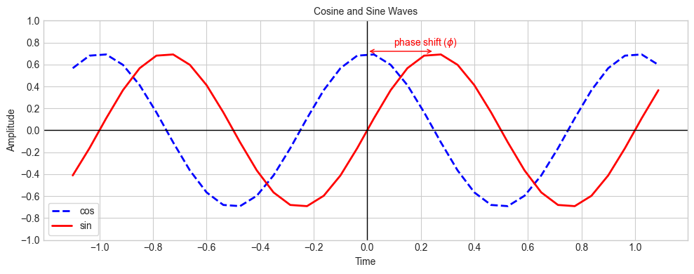
Sine and Cosine Waves

Mathematically, a sinusoidal signal in continuous-time can be represented as: $\( x(t) = A \sin(\omega_0 t + \phi) \)$

While in the digital domain, we express the frequency of the signal with the $\( x[n] = A \sin\left(\frac{2\pi}{N}n + \phi\right) \)$

In Python, we can generate a sinusoidal signal using the np.sin() function from the NumPy library.

x[n] = A * np.sin(2 * np.pi * f0 * t + phi)

• sin represents a cosine wave, and sin represents a sine wave.

• A is the amplitude of the waves.

• f0 is the frequency of the waves in Hertz.

• t is the time axis.

Simply by replacing np.sin() with np.cos(), we can generate a cosine wave.

x[n] = A * np.cos(2 * np.pi * f0 * t + phi)

# Define a signal with amplitude, frequency, phase, and sample rate
A= .7       # Amplitude
f0= 1       # Frequency
phi= 0      # Phase
fs= 16      # Sampling rate

# Define a time vector
t = np.arange(-1.1, 1.1, 1.0 / fs)

cos = A * np.cos(2 * np.pi * f0 * t + phi)
sin = A * np.sin(2 * np.pi * f0 * t + phi)

fig = plt.figure(figsize=(10, 4))
plt.plot(t, cos, 'b', lw=2, label='cos', linestyle='--')
plt.plot(t, sin, 'r', lw=2, label='sin')
plt.xticks(np.arange(-1, 1.1, 0.2))
plt.yticks(np.arange(-1, 1.1, 0.2))

plt.axvline(x=0, color='k', linestyle='solid', linewidth=1)
plt.axhline(y=0, color='k', linestyle='solid', linewidth=1)
plt.text(0.1, 0.8, 'phase shift ($\\phi$)', fontsize=10, verticalalignment='center', color='r')
arrow_style = patches.FancyArrowPatch((0., 0.72), (0.25, 0.72), color='r', mutation_scale=10, arrowstyle='<->')
plt.gca().add_patch(arrow_style)
plt.legend(loc='best', fontsize=10)
plt.xlabel('Time', fontsize=10)
plt.ylabel('Amplitude', fontsize=10)
plt.title('Cosine and Sine Waves', fontsize=10)
plt.grid(True)
plt.tight_layout()
plt.show()