Complex Numbers

import matplotlib.pyplot as plt
import numpy as np

plt.style.use('seaborn-v0_8-whitegrid')
plt.rcParams['legend.frameon'] = True

# # Set global parameters for legend text color, facecolor, and edgecolor
# plt.rcParams['legend.labelcolor'] = 'black'
# plt.rcParams['legend.edgecolor'] = 'black'  # Set to match the color of axis labels

---------------------------------------------------------------------------
ModuleNotFoundError                       Traceback (most recent call last)
Cell In[1], line 1
----> 1 import matplotlib.pyplot as plt
      2 import numpy as np
      4 plt.style.use('seaborn-v0_8-whitegrid')

ModuleNotFoundError: No module named 'matplotlib'

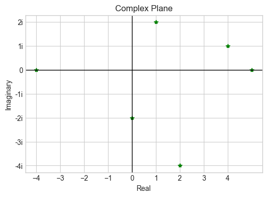
# Generate a range of complex numbers
data = np.array([1+2j, 2-4j, -2j, -4, 4+1j, 5])
x = data.real           # extract real part using numpy array
y = data.imag           # extract imaginary part using numpy array

plt.figure(figsize=(6, 4))
plt.plot(x, y, 'g*')
plt.axvline(x=0, color='k', linestyle='solid', linewidth=1)
plt.axhline(y=0, color='k', linestyle='solid', linewidth=1)
plt.xlabel('Real')
plt.ylabel('Imaginary')
limit=np.max(np.ceil(np.absolute(data))) # set limits for axis
plt.xlim((-limit,limit))
plt.ylim((-limit,limit))
ytick_labels = ['-4i','-3i','-2i','-1i', '0','1i','2i','3i','4i']
ticks = np.array([-4,-3,-2,-1,0,1,2,3,4])
plt.yticks(ticks, ytick_labels)
plt.xticks(ticks)
plt.title('Complex Plane')
plt.grid(True)
plt.axis('equal')  # Equal aspect ratio
plt.show()

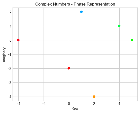
# Calculate phase information
phase = np.angle(data)

# Plot with color representing phase
plt.scatter(x, y, c=phase, cmap='hsv', marker='o')

# Add axis labels
plt.xlabel('Real')
plt.ylabel('Imaginary')

# Add plot title
plt.title('Complex Numbers - Phase Representation')

# Show the plot
plt.show()

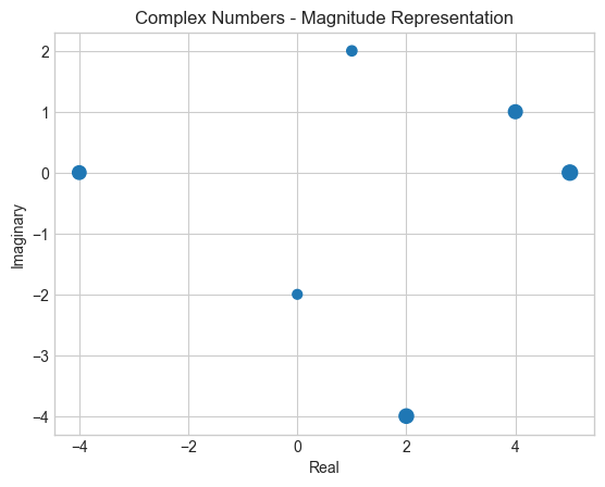
# Calculate magnitude information
magnitude = np.abs(data)

# Scale the marker size based on magnitude
scaled_size = 100 * magnitude / np.max(magnitude)
plt.scatter(x, y, s=scaled_size, marker='o')

# Add axis labels
plt.xlabel('Real')
plt.ylabel('Imaginary')

# Add plot title
plt.title('Complex Numbers - Magnitude Representation')

# Show the plot
plt.show()

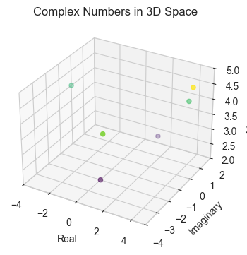
from mpl_toolkits.mplot3d import Axes3D

# Generate complex numbers
data = np.array([1+2j, 2-4j, -2j, -4, 4+1j, 5])

# Extract real and imaginary parts
x = data.real
y = data.imag

# Calculate magnitude for the z-axis
z = np.abs(data)

fig = plt.figure(figsize=(6, 4))
ax = fig.add_subplot(111, projection='3d')

ax.scatter(x, y, z, c=z, cmap='viridis', marker='o')

ax.set_xlabel('Real')
ax.set_ylabel('Imaginary')
ax.set_zlabel('Magnitude')

# Adjust axis limits
ax.set_xlim([min(x), max(x)])
ax.set_ylim([min(y), max(y)])
ax.set_zlim([min(z), max(z)])

# # Move labels into the visible range
# ax.xaxis.labelpad = 10
# ax.yaxis.labelpad = 10
# ax.zaxis.labelpad = 10

plt.title('Complex Numbers in 3D Space')
# plt.tight_layout()
plt.show()

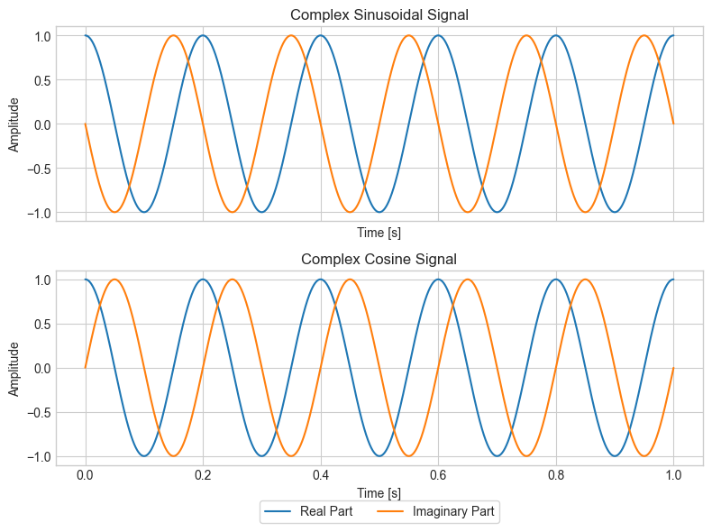
# Parameters for the complex sinusoidal signal
frequency = 5  # Frequency of the sinusoidal signal in Hz (A4 note)
duration = 1.0   # Duration of the signal in seconds
sampling_rate = 44100  # Sampling rate in Hz
phi = 0

# Time array
t = np.linspace(0, duration, int(sampling_rate * duration), endpoint=False)

# Generate a complex sinusoidal signal
sine = np.exp(-1j * 2 * np.pi * frequency * t + phi)
cosine = np.exp(1j * 2 * np.pi * frequency * t + phi)

fig, ax = plt.subplots(figsize=(8, 6), nrows=2, sharex=True)
ax[0].plot(t, np.real(sine), label='Real Part')
ax[0].plot(t, np.imag(sine), label='Imaginary Part')
ax[0].set_title('Complex Sinusoidal Signal')

ax[1].plot(t, np.real(cosine), label='Real Part')
ax[1].plot(t, np.imag(cosine), label='Imaginary Part')
ax[1].set_title('Complex Cosine Signal')

for a in ax:
    a.set_xlabel('Time [s]')
    a.set_ylabel('Amplitude')
    a.grid(True)

plt.legend(loc='upper center', bbox_to_anchor=(0.5, -0.15), ncol=2)
plt.tight_layout()
plt.show()