Sound Waves

import numpy as np
import matplotlib.pyplot as plt
import pandas as pd

plt.style.use('seaborn-v0_8-whitegrid')
plt.rcParams['axes.grid'] = True
np.random.seed(42)

---------------------------------------------------------------------------
ModuleNotFoundError                       Traceback (most recent call last)
Cell In[1], line 1
----> 1 import numpy as np
      2 import matplotlib.pyplot as plt
      3 import pandas as pd

ModuleNotFoundError: No module named 'numpy'

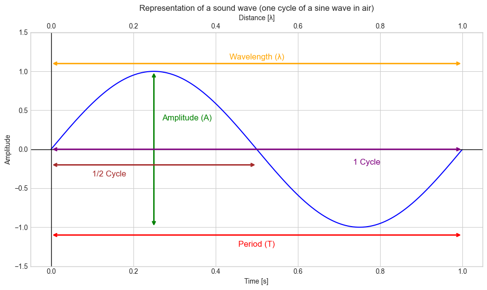
# Define sine wave parameters
A = 1         # Amplitude
f = 1         # Frequency in Hz (1 cycle per second)
T = 1 / f     # Period (seconds per cycle)
λ = T         # Wavelength (assuming speed of wave = 1 unit/s)

# Time vector for one cycle
t = np.arange(0, T, 1/1000)
y = A * np.sin(2 * np.pi * f * t)

# Create figure and axis
fig, ax = plt.subplots(figsize=(10, 6))

# Time domain plot
ax.plot(t, y, 'b', label=r'$y(t) = A \sin(2\pi ft)$')
ax.set_xlabel('Time [s]')
ax.set_ylabel('Amplitude')
ax.set_title('Representation of a sound wave (one cycle of a sine wave in air)')

# Add secondary x-axis for distance
secax = ax.secondary_xaxis('top', functions=(lambda x: x / λ, lambda x: x * λ))
secax.set_xlabel('Distance [λ]')

# Adjust y-limits to make space for annotations
ax.set_ylim(-1.5, 1.5)

# --- Annotations ---

# Amplitude annotation (Vertical arrow from -A to A)
ax.annotate('', xy=(T/4, A), xytext=(T/4, -A), 
            arrowprops=dict(arrowstyle='<->', color='green', lw=2))
ax.text(T/4 + 0.02, 0.4, 'Amplitude (A)', color='green', fontsize=12, va='center')

# Period annotation (Horizontal arrow BELOW the x-axis)
ax.annotate('', xy=(0, -1.1), xytext=(T, -1.1), 
            arrowprops=dict(arrowstyle='<->', color='red', lw=2))
ax.text(T/2, -1.25, 'Period (T)', color='red', fontsize=12, ha='center')

# Wavelength annotation (Horizontal arrow ABOVE the upper x-axis)
ax.annotate('', xy=(0, 1.1), xytext=(λ, 1.1), 
            arrowprops=dict(arrowstyle='<->', color='orange', lw=2))
ax.text(λ/2, 1.15, 'Wavelength (λ)', color='orange', fontsize=12, ha='center')

# 1-cycle annotation (Horizontal arrow BELOW the period annotation)
ax.annotate('', xy=(0, 0), xytext=(T, 0), 
            arrowprops=dict(arrowstyle='<->', color='purple', lw=2))
ax.text(0.8, -0.2, '1 Cycle', color='purple', fontsize=12, ha='right')

# Half-cycle annotation (Horizontal arrow BELOW the 1-cycle annotation)
ax.annotate('', xy=(0, -0.2), xytext=(T/2, -0.2), 
            arrowprops=dict(arrowstyle='<->', color='brown', lw=2))
ax.text(0.1, -0.35, '1/2 Cycle', color='brown', fontsize=12, ha='left')

# Formatting
ax.axhline(0, color='black', linewidth=1)
ax.axvline(0, color='black', linewidth=1)
plt.tight_layout()
plt.show()

Frequency (\(f\)) is a crucial parameter. It tells us how many cycles of the waveform occur in one second.

It’s the inverse of the period (\(T\)), where \(T\) is the time taken for one complete cycle. The relationship between frequency and period is given by: $\( f = \frac{1}{T} \quad \text{and} \quad T = \frac{1}{f} \)$

Wavelength is calculated using the speed of sound \( c_{air} = 343 m/s\) and the frequency of the sound wave. The relationship between wavelength and frequency is given by:

\[ \lambda = \frac{c_{air}}{f} \]

# Data for frequency and corresponding wavelengths
frequencies = [
    20, 25, 31.5, 40, 50, 63, 80, 100, 125, 160, 200, 250, 315, 400, 500, 630,
    800, 1000, 1250, 1600, 2000, 2500, 3150, 4000, 5000, 6300, 8000, 10000, 12500,
    16000, 20000
]
wavelengths = [
    17.15, 13.72, 10.90, 8.58, 6.86, 5.44, 4.29, 3.43, 2.75, 2.14, 1.72, 1.37,
    1.09, 0.86, 0.69, 0.54, 0.43, 0.34, 0.27, 0.21, 0.17, 0.14, 0.11, 0.086,
    0.069, 0.054, 0.043, 0.034, 0.027, 0.021, 0.017
]

# Create DataFrame
df = pd.DataFrame({
    'Frequency (Hz)': frequencies,
    'Wavelength (m)': wavelengths
})

# Display the table
df

	Frequency (Hz)	Wavelength (m)
0	20.0	17.150
1	25.0	13.720
2	31.5	10.900
3	40.0	8.580
4	50.0	6.860
5	63.0	5.440
6	80.0	4.290
7	100.0	3.430
8	125.0	2.750
9	160.0	2.140
10	200.0	1.720
11	250.0	1.370
12	315.0	1.090
13	400.0	0.860
14	500.0	0.690
15	630.0	0.540
16	800.0	0.430
17	1000.0	0.340
18	1250.0	0.270
19	1600.0	0.210
20	2000.0	0.170
21	2500.0	0.140
22	3150.0	0.110
23	4000.0	0.086
24	5000.0	0.069
25	6300.0	0.054
26	8000.0	0.043
27	10000.0	0.034
28	12500.0	0.027
29	16000.0	0.021
30	20000.0	0.017