Linear Algebra Basics with Numpy#
Basic linear algebra operations to practice with numpy. Inspired by this tutorial.
import numpy as np
import matplotlib.pyplot as plt

plt.style.use('default')
plt.rcParams['legend.frameon'] = True
---------------------------------------------------------------------------
ModuleNotFoundError                       Traceback (most recent call last)
Cell In[1], line 1
----> 1 import numpy as np
      2 import matplotlib.pyplot as plt
      4 plt.style.use('default')

ModuleNotFoundError: No module named 'numpy'
Vectors#
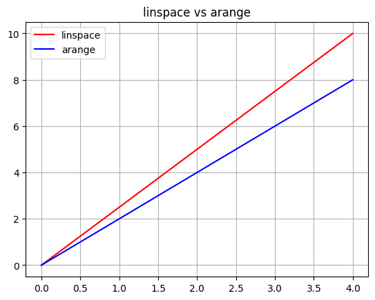
What is the difference between np.linspace and np.arange?
vec_linspace = np.linspace(0, 10, 5) # 5 points between 0 and 10 evenly spaced
vec_arange = np.arange(0, 10, 2) # 5 points between 0 and 10 with step 2

print('first:', vec_linspace, 'second:', vec_arange)
print(type(vec_linspace), type(vec_arange))
first: [ 0.   2.5  5.   7.5 10. ] second: [0 2 4 6 8]
<class 'numpy.ndarray'> <class 'numpy.ndarray'>
plt.plot(vec_linspace, 'r', label='linspace')
plt.plot(vec_arange, 'b', label='arange')
plt.title('linspace vs arange')
plt.legend()
plt.grid(True)
plt.show()
Dot Product#
The two vectors must have the same length.
The dot product is the sum of the products of the corresponding elements of the two vectors.
It is alwatys a scalar.
vector1 = np.array([1, 2, 3])
vector2 = np.array([4, 5, 6])

print('dot product:', np.dot(vector1, vector2))
dot product: 32
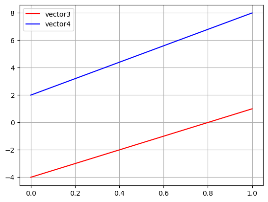
# orthogonal vectors
print('Two vectors are orthogonal if their dot product is zero.')
vector3 = np.array([-4, 1])
vector4 = np.array([2, 8])
print('dot product:', np.dot(vector3, vector4))
Two vectors are orthogonal if their dot product is zero.
dot product: 0
plt.plot(vector3, 'r', label='vector3')
plt.plot(vector4, 'b', label='vector4')
plt.legend()
plt.grid(True)
plt.show()
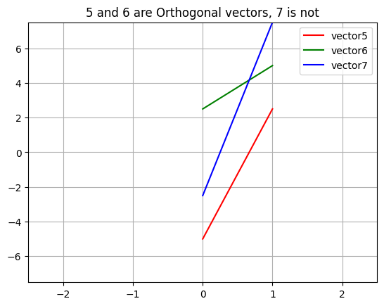
# orthogonal vectors
vector5 = np.array([-5, 2.5])
vector6 = np.array([2.5, 5])
vector7 = np.array([-2.5, 7.5])
print('dot product <5,6>:', np.dot(vector5, vector6))
print('dot product <5,7>:', np.dot(vector5, vector7))
print('dot product <6,7>:', np.dot(vector6, vector7))

plt.title('5 and 6 are Orthogonal vectors, 7 is not')
plt.plot(vector5, 'r', label='vector5')
plt.plot(vector6, 'g', label='vector6')
plt.plot(vector7, 'b', label='vector7')
plt.xlim(-2.5, 2.5)
plt.ylim(-7.5, 7.5)
plt.legend()
plt.grid(True)
plt.show()
dot product <5,6>: 0.0
dot product <5,7>: 31.25
dot product <6,7>: 31.25
Transpose of a Vector#
v1 = np.array([2, 3, -1], ndmin=2)
print(v1)
print('')
print(v1.T)
[[ 2  3 -1]]

[[ 2]
 [ 3]
 [-1]]
Matrices definitions#
Define a matrix with np.array.
Let’s call it M_0.
M_0 = np.array([[1, 2, 3], [4, 5, 6], [7, 8, 9]])
print('Matrix: \n', M_0, '\n','type:', type(M_0),'\n', 'shape:', np.shape(M_0))
Matrix:
 [[1 2 3]
 [4 5 6]
 [7 8 9]]
 type: <class 'numpy.ndarray'>
 shape: (3, 3)
Generate an identity matrix of 3 by 3 with np.eye.
I_3 = np.eye(3)
print('Identity matrix: \n', I_3, '\n','type:', type(I_3),'\n', 'shape:', np.shape(I_3))
Identity matrix:
 [[1. 0. 0.]
 [0. 1. 0.]
 [0. 0. 1.]]
 type: <class 'numpy.ndarray'>
 shape: (3, 3)
Initialize a matrix with zeros with np.zeros.
np.zeros((3, 4))
array([[0., 0., 0., 0.],
       [0., 0., 0., 0.],
       [0., 0., 0., 0.]])
Generate a matrix of specifed size and filled with a number we declare with np.full.
np.full((5, 2), 7)
array([[7, 7],
       [7, 7],
       [7, 7],
       [7, 7],
       [7, 7]])
Matrices operations#
A few operations are available for matrices:
Scalar matrix multiplication
Transpose of a square matrix
Transpose of a rectangular matrix
# scalar matrix multiplication
M_1 = np.array([[2, 3], [4, 5]]) # mind the outer brackets !
M_2 = np.array([[1, 6], [7, 8]])
M_res = np.dot(M_1, M_2)
print(M_1)
print('')
print(M_2)
print('')
print('Matrix multiplication: \n', M_res)
[[2 3]
 [4 5]]

[[1 6]
 [7 8]]

Matrix multiplication:
 [[23 36]
 [39 64]]
# Transpose of a square matrix
M_rnd = np.random.randint(0, 10, (3, 3))
print(M_rnd)
print('')
print(M_rnd.T)
MT = M_rnd.T
print('')
print(MT.T)
[[0 3 9]
 [6 2 3]
 [8 9 0]]

[[0 6 8]
 [3 2 9]
 [9 3 0]]

[[0 3 9]
 [6 2 3]
 [8 9 0]]
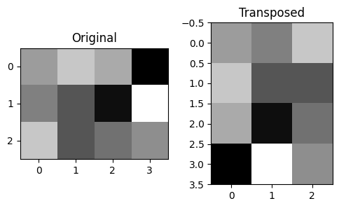
# Transpose of a rectangular matrix
M_rect = np.random.randint(0, 20, (3, 4))
print(M_rect)
print('')
print(M_rect.T)

fig, ax = plt.subplots(1, 2, figsize=(6, 3))
ax[0].imshow(M_rect, cmap='gray')
ax[0].set_title('Original')
ax[1].imshow(M_rect.T, cmap='gray')
ax[1].set_title('Transposed')
[[12 15 13  1]
 [10  7  2 19]
 [15  7  9 11]]

[[12 10 15]
 [15  7  7]
 [13  2  9]
 [ 1 19 11]]
Text(0.5, 1.0, 'Transposed')
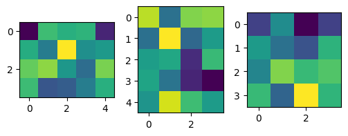
Matrix multiplication with numpy @ operator and np.matmul.
# Matrix multiplication with numpy @ operator and np.matmul
M3 = np.random.randn(4,5)
M4 = np.random.randn(4,5)
print(np.matmul(M3, M4.T))
print('')
print(M3 @ M4.T)
print('')
print(np.matmul(M3, M4.T) - M3 @ M4.T)

fig, ax = plt.subplots(1, 3, figsize=(6, 2))
ax[0].imshow(M3)
ax[1].imshow(M4.T)
ax[2].imshow(M3 @ M4.T)
plt.show()
[[-2.50497566  0.04954823 -4.1938966  -2.50645707]
 [ 0.53563016 -0.94366116 -1.97548804  1.41066921]
 [-0.23106035  2.86184088  1.65311328  2.15090219]
 [ 1.66203211 -1.39785448  4.49946399  1.50330059]]

[[-2.50497566  0.04954823 -4.1938966  -2.50645707]
 [ 0.53563016 -0.94366116 -1.97548804  1.41066921]
 [-0.23106035  2.86184088  1.65311328  2.15090219]
 [ 1.66203211 -1.39785448  4.49946399  1.50330059]]

[[0. 0. 0. 0.]
 [0. 0. 0. 0.]
 [0. 0. 0. 0.]
 [0. 0. 0. 0.]]
Matrix multiplication with identity matrix.
I = np.eye(3, dtype=int) # identity matrix of 3 by 3
M5 = np.random.randint(0, 10, (3, 3))
print('identity matrix:')
print(I)
print('our random int mtx:')
print(M5)
print('matrix multiplication of I and M5:')
print(I @ M5)
identity matrix:
[[1 0 0]
 [0 1 0]
 [0 0 1]]
our random int mtx:
[[7 1 4]
 [9 0 5]
 [0 4 8]]
matrix multiplication of I and M5:
[[7 1 4]
 [9 0 5]
 [0 4 8]]
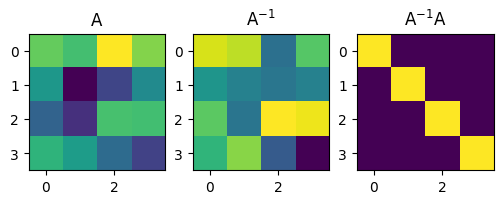
Why a matrix inverse is necessary ?#
Matrix division is not possible, but we can use the inverse of a matrix to solve a system of linear equations: $\( A x = b \)$
We can rewrite this as: $\( A^{-1} A x = A^{-1} b \)$
And then, using the fact that the inverse of a matrix multiplied by the matrix itself is the identity matrix: $\(I x = A^{-1} b\)$
And finally we can solve for x: $\(x = A^{-1} b\)$
A = np.random.randn(4,4)
Ainv = np.linalg.inv(A)

AinvA = Ainv @ A

print(A)
print('')
print(AinvA)
[[ 0.84155985  0.62139304  1.66641305  1.02123927]
 [ 0.01715069 -1.8241851  -1.0945571  -0.15466435]
 [-0.71343633 -1.3434311   0.64798847  0.60942635]
 [ 0.4490001   0.11109018 -0.59911332 -1.14225656]]

[[ 1.00000000e+00 -2.54575514e-16  1.23158986e-16 -1.78836882e-17]
 [-2.74744330e-17  1.00000000e+00  1.01355464e-16  9.18656809e-17]
 [ 1.08638722e-17 -4.29486708e-17  1.00000000e+00 -1.75831950e-16]
 [ 3.30848099e-18 -7.42051923e-17  5.09021073e-17  1.00000000e+00]]
fig, ax = plt.subplots(1, 3, figsize=(6, 2))
ax[0].imshow(A)
ax[0].set_title('A')
ax[1].imshow(Ainv)
ax[1].set_title('A$^{-1}$')
ax[2].imshow(AinvA)
ax[2].set_title('A$^{-1}$A')
plt.show()
Create a 3x3 vector, create a diagonal matrix from it
v = np.array([1, 2, 3])
D = np.diag(v) # diagonal matrix from vector v
print(D)
[[1 0 0]
 [0 2 0]
 [0 0 3]]
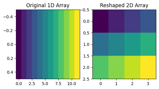
Manipulation of matrices#
# Create a simple 1D array
original_array = np.arange(12)

# Reshape the array to a 2D matrix (3 rows, 4 columns)
reshaped_array = original_array.reshape(3, 4)

# Visualize the original and reshaped arrays using imshow
plt.figure(figsize=(6, 3))
plt.subplot(1, 2, 1)
plt.imshow(original_array.reshape(1, -1), cmap='viridis', aspect='auto')
plt.title('Original 1D Array')

plt.subplot(1, 2, 2)
plt.imshow(reshaped_array, cmap='viridis', aspect='auto')
plt.title('Reshaped 2D Array')

plt.show()
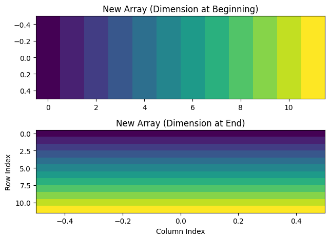
# Add a dimension at the beginning
new_array_beginning = original_array[np.newaxis, :]

# Add a dimension at the end
new_array_end = original_array[:, np.newaxis]

print(f"original array shape: {original_array.shape}")
print(original_array)
print("")
print(f"new array with dim at beginning shape: {new_array_beginning.shape}")
print(new_array_beginning)
print("")
print(f"new array with dim at end shape: {new_array_end.shape}")
print(new_array_end)
original array shape: (12,)
[ 0  1  2  3  4  5  6  7  8  9 10 11]

new array with dim at beginning shape: (1, 12)
[[ 0  1  2  3  4  5  6  7  8  9 10 11]]

new array with dim at end shape: (12, 1)
[[ 0]
 [ 1]
 [ 2]
 [ 3]
 [ 4]
 [ 5]
 [ 6]
 [ 7]
 [ 8]
 [ 9]
 [10]
 [11]]
Difference between adding a dimension at the beginning or at the end of a matrix.
plt.subplot(2, 1, 1)
plt.imshow(new_array_beginning, cmap='viridis', aspect='auto')
plt.title('New Array (Dimension at Beginning)')

plt.subplot(2, 1, 2)
plt.imshow(new_array_end, cmap='viridis', aspect='auto')
plt.title('New Array (Dimension at End)')
plt.xlabel('Column Index')
plt.ylabel('Row Index')

plt.tight_layout()
plt.show()
Difference between np.array and np.matrix#
In NumPy, both np.array and np.matrix are used to represent matrices, but there are some key differences between them.
Type:#
np.array: It represents a general n-dimensional array. Arrays can have any number of dimensions, and they are the more commonly used data structure in NumPy.
np.matrix: It represents a specialized 2-dimensional matrix. Matrices are a subclass of arrays and provide some additional features specifically designed for linear algebra operations.
Multiplication:#
np.array: The * operator performs element-wise multiplication.
np.matrix: The * operator performs matrix multiplication, which is equivalent to the dot function.
Power Operator (**):#
np.array: The ** operator performs element-wise exponentiation.
np.matrix: The ** operator performs matrix exponentiation.
Matrix Specific Methods:#
np.array: Arrays have a broader range of methods and functions available, but they don’t have methods specific to matrix operations.
np.matrix: Matrices have specific methods like I for matrix inversion, H for conjugate transpose, and A for matrix data.
Creation:#
np.array: Arrays are created using the np.array function.
np.matrix: Matrices are created using the np.matrix function or by using np.array with ndmin=2 parameter.
# Creating arrays
array_a = np.array([[1, 2], [3, 4]])
array_b = np.array([[5, 6], [7, 8]])

# Creating matrices
matrix_a = np.matrix([[1, 2], [3, 4]])
matrix_b = np.matrix([[5, 6], [7, 8]])

# Element-wise multiplication
array_result = array_a * array_b

# Matrix multiplication
matrix_result = matrix_a * matrix_b

print("Array multiplication:")
print(array_result)

print("\nMatrix multiplication:")
print(matrix_result)
Array multiplication:
[[ 5 12]
 [21 32]]

Matrix multiplication:
[[19 22]
 [43 50]]